CLM-FATES and CLM Perturbed Parameter Ensemble
About this Study
This interactive app explores how individual parameter perturbations affect model outputs in the CLM and CLM-FATES models in Satellite Phenology (SP) mode. Each parameter is varied one at a time to assess its influence on key biophysical variables.
How to Use This App
Each tab in the app focuses on a specific way to explore and interpret the one-at-a-time parameter ensemble results:
-
Parameter Explorer:
Lets you select individual parameters to see how they affect model outputs.
-
Ensemble Variance:
Provides a high-level look at ensemble ranges and variance for both models.
-
Top Parameters:
Lets you look at the most influential parameters on different model outputs.
-
Model Comparison:
Compares the CLM and CLM-FATES responses side by side for equivalent parameter perturbations.
-
Parameter Information:
Searchable table of parameter names and descriptions.
-
Download Data:
Download data from this study.
Use the navigation bar above to switch between sections. Hover over plots for details, and use the download buttons to save data or figures.
Methods
High-level summary of CLM and CLM-FATES models:
-
CLM 6.0 (Community Land Model):
Simulates terrestrial energy, water, and carbon fluxes.
-
CLM-FATES (Functionally Assembled Terrestrial Ecosystem Simulator):
Adds a detailed representation of vegetation structure and function.
Both models were run in satellite phenology (SP) mode, where canopy structure (LAI, SAI, height) is prescribed from satellite observations.
When CLM is coupled to FATES, CLM provides site and soil conditions and atmospheric forcing, while FATES simulates plant physiological, vegetation demography, and biogeochemical processes (Fig. 1).
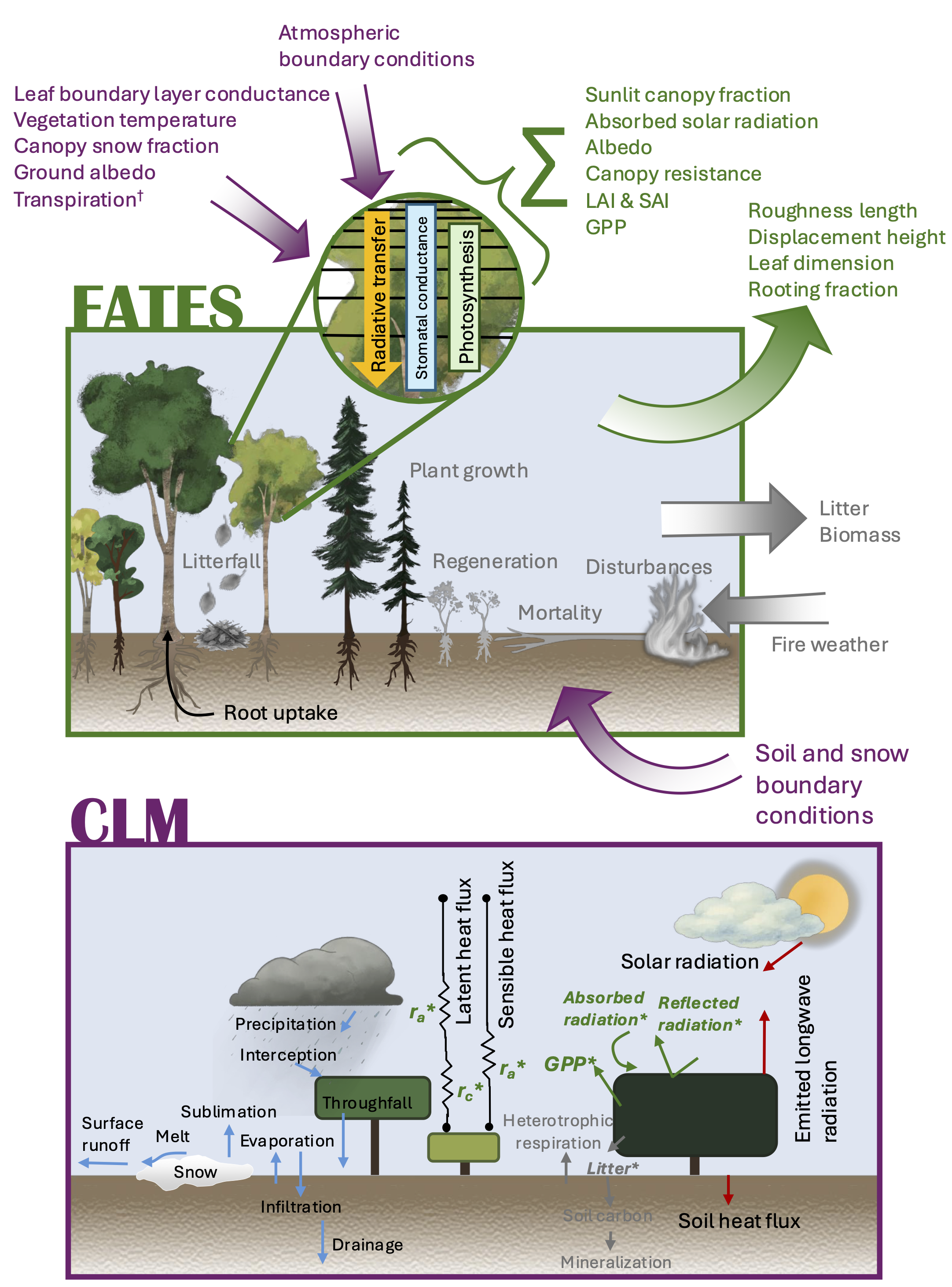 Figure 1: Processes simulated in CLM-FATES by each model. Top: processes simulated by FATES when connected to CLM. Arrows in purple indicate conditions supplied to FATES by CLM. Arrows in green indicate conditions supplied to CLM by FATES. Anything in gray is not active in SP mode. Bottom: Processes simulated by CLM when connected to FATES. Green starred variables are simulated and provided by FATES or in the case of aerodynamic resistance (ra) are influenced by the FATES-provided roughness length, displacement height, and leaf dimension. Items in gray are not active in SP mode. †: Only used in FATES hydraulics mode, which is not utilized in this study.
For more details, see
CLM documentation
and
FATES documentation
.
Both CLM and CLM-FATES were run in SP mode using prescribed GSWP3 meteorology (2000–2014).
A 45-year spinup ensured stable soil and energy conditions, and results from an additional 15 years were analyzed.
To reduce computational cost, we used a 400-point ‘sparse grid’ that represents global variability following
Kennedy et al. (2025)
. (Fig. 2)
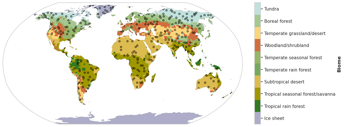 Figure 2: Locations of the 400 sparse grid cells, along with Whittaker biome.
We tested how individual parameter changes affect model outputs using one-at-a-time parameter perturbations.
- Each parameter was run at its minimum and maximum value.
- Parameter ranges were derived from literature, expert judgment, and prior PPEs.
- In total: 204 CLM parameters and 137 FATES parameters were perturbed.
- Parameters were grouped as common, CLM-only, or FATES-only.
Vegetation-related parameters were perturbed together across all PFTs to limit simulation count.
Contact
Adrianna Foster, NCAR —
afoster@ucar.edu
Citations
If you use this data or figures please cite the paper associated with the project:
Foster, A., Hawkins, L. R., Kennedy, D., Bonan, G., Fisher, R.,
Needham, J., Knox, R., Koven, C., Wieder, W., Dagon, K., &
Lawrence, D. (2026). Contrasting parametric sensitivities
in two global vegetation models using parameter perturbation
ensembles [Data set]. In Journal of Advances in Modeling Earth Systems.
Zenodo
https://doi.org/10.5281/zenodo.18203140
You can also find the full dataset associated with this project at:
Foster, A., Hawkins, L. R., Kennedy, D., Bonan, G., Fisher, R.,
Needham, J., Knox, R., Koven, C., Wieder, W., Dagon, K., &
Lawrence, D. (2026). Contrasting parametric sensitivities
in two global vegetation models using parameter perturbation
ensembles [Data set]. In Journal of Advances in Modeling Earth Systems.
Zenodo
https://doi.org/10.5281/zenodo.18203140
Acknowledgments
This material is based upon work supported by the NSF National Center for Atmospheric Research, which is a major facility sponsored by the National Science Foundation under Cooperative Agreement No. 1852977. Computing and data storage resources, including the Derecho supercomputer (doi:10.5065/qx9a-pg09) were provided by the Climate Simulation Laboratory at NSF-NCAR's Computational and Information Systems Laboratory (CISL).